Fluid Simulation Tutorial

Fluid Tutorial

This tutorial walks you through the advection and projection steps of simulating incompressible fluids on a grid. The algorithm follows the approach described in "SIGGRAPH 2007 Course notes on fluids" by Robert Bridson and Matthias Muller-Fischer.

This tutorial walks you through using a staggered MAC Grid as well as your first advection step and projection steps. I provide computed values which you can then compare against your own code.

The most important milestone for fluid simulation is creating a stable, divergence free velocity field. Once the velocity field is stable, it is simple to advect arbitrary quantities within the grid, such as smoke density, heat, color, or whatever. By divergence free, we mean

the volume of each cell remains constant each time step
the velocity entering each cell should equal the velocity leaving each cell
if we sum the rates of change in velocity in every direction, they should sum to zero, e.g. \[ \nabla \cdot u = \frac{du}{dt} + \frac{dv}{dt} + \frac{dw}{dt} = 0 \]

MAC Grid

Our first step is to understand the MAC Grid structure. The MAC Grid is a data structure for discretizing the space of our fluid. Quantities in the world, such as velocities and smoke density, will be stored at cell faces and centers. We use a staggered MAC Grid in particular because it allows us to estimate the derivatives (e.g. the rates of change in each direction) with more numerical stability (read the Bridson/Muller-Fischer notes to understand why!).

To start with something simple, create a 2x2x1 MAC grid as follows.


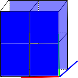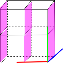
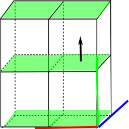
X faces are used to store the u-component of the velocity.	Y faces are used to store the v-component of the velocity.	Z faces are used to store the w-component of the velocity.

In our small MAC Grid above, we have 4 cells, 8 Z faces, 6 Y faces, and 6 X faces. We will store velocities at the faces and other quantities, such as smoke density, at the cell centers. Specifically, if we define the velocities with (u,v,w), we store the u values at X-faces, v values are Y-faces, and w values at Z-faces. The only tricky thing to remember is that we will need to compute the full velocity (u,v,w) at each face location, but then only store one of the components there. Implementation-wise, we have separate arrays, mU, mV, and mW for storing each velocity component. (i,j,k) indexing is used for each array of faces, for example,

The front Z face indices are (1,1,0)(0,1,0)(1,0,0)(0,0,0). The back Z face indices are (1,1,1)(0,1,1)(1,0,1)(0,0,1).
The Y face indices are (0,0,0),(0,1,0),(0,2,0) and (1,0,0)(1,1,0)(1,2,0).
The X face indices are (0,0,0),(0,1,0) and (1,0,0),(1,1,0) and (2,0,0)(2,1,0).

In the code, indices in the Z direction correspond to rows and are indexed with i; indices in the Y direction correspond to stacks and are indexed with j; and indices in the X direction correspond to columns and are indexed with i. Next, we will compute a single advection and project step.

Advection

An empty MAC Grid, where all values are zero, corresponds to a grid with no velocity in it. Our first step is to add some movement to shake things up. To simplest way to start is to add a non-zero velocity to one of the internal faces of the grid. Let's add 1 unit of velocity in the Y direction, e.g. mV(0,1,0) = 1.

What is the velocity at the center of each cell? Either (0,0,0) or (0,0.5,0)

Now that we've added some source velocity to the grid, we perform an advection step. Again, please refer to the notes if you're not sure of the details. Briefly, we go through each face in the grid and traceback to fetch the velocity that will be at our current location next step.

    FOR_EACH_FACE
        currentpt = position at center of current face
        currentvel = velocity at center of current face 
        oldpt = currentpt - dt * currentvel
        newvel = velocity at old location
        store one component of newvel depending on face type

Computing the velocities at arbitrary places in the grid is done by interpolating between the values stored at each face.

What is the position of the Y-face? (0.5,1.0,0.5)
What is oldpt? (0.5,1.0,0.5) - (0.1)*(0,1,0) = (0.5, 0.9, 0.5)
What is the velocity at position (0.5,0.9,0.5)? (0,0.9,0)
What is the new value of mV(0,1,0)? 0.9

Notes:

Because of traceback and interpolation, we never get a velocity that is larger than the values stored on the grid. This results in dissapation and loss of detail, but ensures that the system stays stable. Detail and dissapation can be counteracted by adding additional forces such as vorticity confinement.
Parameter tweaking tip: make sure your timestep and velocities are not too large. In particular, you never want your traceback step to be larger than your grid size.
What should you do when your traceback step takes you outside of the grid? If the position corresponds to a fluid source, just return the source value. You can also extrapolate the velocity from the nearest boundary, or set the value to zero (although this results in greater dissappation near boundaries)

Projection

After advecting the velocity, we can add external forces -- such as gravity, buoyancy, and vorticity confinement -- using a straight-forward euler step. Now, we have a new velocity field, but there's only one problem! It's not divergence free so anything we try to do to it will blow up. In this step, we will compute pressures so that when we apply them to the field the divergence-free property holds.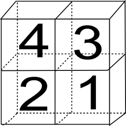

We will compute pressure values at the center of each cell which ensure that the resulting velocity field is divergence free.

The SIGGRAPH fluid course notes give a good description of the derivation of the Poisson equations that we will use to solve for pressure. To summarize, the values of our fluid at the next time step can be described in terms of our current (divergent, unstable) velocity field and the pressure, \[ u^{n+1}= u^* - \delta t \frac{1}{\rho} \nabla p \] where \(u^*\) is our current velocity field, \(\rho\) is the fluid pressure and is a parameter set by the user. In the above equation, the pressures are unknown. What should they be? We want the pressures that satisfy \[ \nabla \cdot u = 0 \] In other words, we want the rates of change in each direction of the cell to sum to zero, e.g. the amount of velocity entering the cell equals the amount leaving, e.g. \[ \nabla \cdot u = \frac{du}{dt} + \frac{dv}{dt} + \frac{dw}{dt} = 0 \] where each of the derivatives above can be easily computed using finite differences between the faces on our grid. For example, to compute du/dt, we subtract the values stored at the X faces on each side of the cell and then divide by the cell size. \[ \frac{du}{dt} = \large{\frac{u_{i+\frac{1}{2},j,k} - u_{i-\frac{1}{2},j,k}}{\Delta x}} \] \[ \frac{dv}{dt} = \large{\frac{v_{i,j+\frac{1}{2},k} - v_{i,j-\frac{1}{2},k}}{\Delta y}} \] \[ \frac{dw}{dt} = \large{\frac{w_{i,j,k+\frac{1}{2}} - w_{i,j,k-\frac{1}{2}}}{\Delta z}} \] We will assume that our grid cells are square (e.g. \(\Delta x = \Delta y = \Delta z\)). Now, we can write our divergence equation in terms of our current velocity field. For example, for a fluid cell surrounded by fluid cells, we would get \[ \frac{du}{dt} = \frac{1}{\Delta x} \left[ \left( u^*_{i+\frac{1}{2},j,k} - \frac{\Delta t}{\rho} \left(\frac{p_{i+1,j,k}-p_{i,j,k}}{\Delta x}\right)\right) - \left( u^*_{i-\frac{1}{2},j,k} - \frac{\Delta t}{\rho} \left(\frac{p_{i,j,k}-p_{i-1,j,k}}{\Delta x}\right) \right) \right] \] \[ \frac{dv}{dt} = \frac{1}{\Delta x} \left[ \left( v^*_{i,j+\frac{1}{2},k} - \frac{\Delta t}{\rho} \left(\frac{p_{i,j+1,k}-p_{i,j,k}}{\Delta x}\right)\right) - \left( v^*_{i,j-\frac{1}{2},k} - \frac{\Delta t}{\rho} \left(\frac{p_{i,j,k}-p_{i,j-1,k}}{\Delta x}\right) \right) \right] \] \[ \frac{dw}{dt} = \frac{1}{\Delta x} \left[ \left( w^*_{i,j,k+\frac{1}{2}} - \frac{\Delta t}{\rho} \left(\frac{p_{i,j,k+1}-p_{i,j,k}}{\Delta x}\right)\right) - \left( w^*_{i,j,k-\frac{1}{2}} - \frac{\Delta t}{\rho} \left(\frac{p_{i,j,k}-p_{i,j,k-1}}{\Delta x}\right) \right) \right] \] If we rearrange terms and put all our unknowns on the RHS and knowns on the LHS, we get the following for fluid cells that are surrounded by fluid neighbors. The RHS is the divergence of cell (i,j,k) and is computed with finite differences (just like above!). \[ \left(6 p_{i,j,k} - p_{i+1,j,k} - p_{i-1,j,k} - p_{i,j+1,k} - p_{i,j-1,k} - p_{i,j,k+1} - p_{i,j,k-1} \right) = \frac{-\Delta x^2}{\Delta t \rho} \left( \nabla \cdot u^* \right) \] It's possible to derive similar expressions for fluid cells next to a boundary or solid. In general, the rules are

The coefficient for \(p_{i,j,k}\) is the number of fluid neighbors
The coefficient for fluid neighbors is -1
The coefficient for non neighbors is 0

Finally, we can derive an equation for every fluid cell in the grid. These can be combined into a large system of equations \[ Ap = b \] Each of the rows of A represents the equation for a fluid cell. If we have 4 cells, A is a 4x4 matrix. The 4x1 column vector p is the pressure for each cell (our unknowns). The 1x4 column vector b is a function of the current divergence in each cell. Going back to our concrete example, our system of equations would look like \[ \left[ \begin{array}{cccc} 2 & -1 & -1 & 0 \\ -1 & 2 & 0 & -1 \\ -1 & 0 & 2 & -1 \\ 0 & -1 & -1 & 2\end{array} \right] \left[ \begin{array}{c} p_1 \\ p_2 \\ p_3 \\ p_3\end{array} \right] = -\frac{\Delta x^2}{\Delta t \rho}\left[ \begin{array}{c} \nabla \cdot u_1 \\ \nabla \cdot u_2 \\ \nabla \cdot u_3 \\ \nabla \cdot u_4 \end{array} \right] \] In this example, suppose \(\Delta x = 1, \Delta t = 0.1, \rho = 1\). In this case, b is \[ b = -\frac{(1.0)^2}{(0.1)*(1.0)}\left[ \begin{array}{c} ((0.9-0) + 0 + 0)/1.0\\ 0.0\\ ((0-0.9) + 0 + 0)/1.0 \\ 0.0 \end{array} \right] = \left[ \begin{array}{c} -9\\ 0\\ 9\\ 0\end{array} \right] \] Now, we can plug in this equation into a linear solver such as matlab, to find values for p. It turns out that we get \[ p = \left[ \begin{array}{c} -3.375\\ -1.125\\ 3.375\\ 1.125\end{array} \right] \] Now that we have values for p, we can compute our new velocity field. \[ u_{1,0,0} = u^*_{1,0,0} - \frac{\Delta t}{\Delta x \rho}\left(-1.125 + 3.375 \right) = -0.225 \\ \] \[ u_{1,1,0} = u^*_{1,1,0} - \frac{\Delta t}{\Delta x \rho}\left( 1.125 - 3.375 \right) = 0.225 \\ \] \[ v_{0,1,0} = u^*_{0,1,0} - \frac{\Delta t}{\Delta x \rho}\left( 3.375 + 3.375 \right) = 0.225 \\ \] \[ v_{1,1,0} = u^*_{1,1,0} - \frac{\Delta t}{\Delta x \rho}\left( 1.125 + 1.125 \right) = -0.225 \] Note that from our advection step, \(u^*_{0,1,0} = 0.9\) but all other velocities are 0. Also, we only compute new velocities for our interior faces because the boundary faces correspond to stationary objects and thus have velocity 0. The resulting velocity field swirls around like a pinwheel in the interior of the grid. The contents of mU = {0,-0.225,0,0,0.225,0}, mV = {0,0,0.225,-0.225,0,0}, and mW = {0,0,0,0,0,0,0}.
Notes:

Check that the velocity field after this step is divergence free by computing the divergence at each cell.
If you use a uniform grid size, \(\Delta x = \Delta y = \Delta z\)
What is the velocity normal to a solid border? \(u_{solid}\)
The fluid has free movement tangent to the boundaries.
The resulting velocity field should be look smooth, no sudden changes!

Putting it all together

Once we have a divergence free velocity field, we can advect other properties in the field. For smoke, the fluid we simulate is the air, within which we would advect the smoke density (carefull! the smoke density is different from the air fluid density which we use in the projection step!) or temperature for buoyancy forces. Putting it all together, a typical simulation step might look like

void SmokeSim::step()
{
   double dt = 0.01;

   // Step0: Gather user forces
   mGrid.updateSources();

   // Step1: Calculate new velocities
   mGrid.advectVelocity(dt);
   mGrid.addExternalForces(dt);
   mGrid.project(dt);

   // Step2: Calculate new temperature
   mGrid.advectTemperature(dt);

   // Step3: Calculate new density 
   mGrid.advectDensity(dt);
}

To simulate fire, we can simulate two fluids simultaneously: one for the fuel sources and one for the air. The tricky parts are keeping track of the flame front (e.g. the boundary between the two fluids) and ensuring that mass is preserved with the two fluids coupled together (see "Physically Based Modeling and Animation of Fire"). To simulate explosions, we can modify the projection step so that instead of ensuring the divergence is zero, we solve for a non-zero divergence which estimates the explosion's blast wave (without explicitly simulating it, phew, see "Animating Suspended Particle Explosions"). To simulate water, we need to keep track of the water surface, say with a level set, and handle the interactions between the fluid and air (see the SIGGRAPH notes for a good introduction). And finally, best of luck and happy coding!